PROBABILITY AND STATISTICS
 |
In this unit, you will continue your study of probability by studying how probability can be used to make fair decisions and to analyze decisions. You will also learn how statistics are used to analyze and interpret data.
PROBABILITY |
Using Probabilities to Make a Fair Decision
A fair game is a game in which all participants have an equal chance of winning. Probability can be used to decide whether a game is fair or unfair.
In all examples, a 6-sided number cube or die is used. Die is the singular for dice.
Example #1: Two captains of the baseball team need to determine which team bats first. Team A bats first if an even number is rolled on a die. Team B bats first if an odd number is rolled on a die. Will this method result in a fair decision?
Solution: The probability of rolling an even number is 3/6 = ½. The probability of rolling an odd number is also 3/6 or ½. This is a fair method of determining which team bats first, since there is an equal chance of rolling an even or an odd number.
Example #2: Alli and Ben play a game using a die. Alli gets a point if she rolls a number evenly divisible by 2. Ben gets a point if he rolls a number evenly divisible by 3. Is this a fair game?
Solution: Alli scores a point if she rolls a 2, 4, or 6. The probability of Alli scoring a point is 3/6 = ½. Ben scores a point if he rolls a 3 or a 6. The probability of Ben scoring a point is 2/6 = 1/3. This game is unfair since the probability of Alli scoring a point is greater than the probability of Ben scoring a point.
Example #3: Ella, Brenda and Sarah take turns tossing two coins. Each player receives a point depending on the outcome of the tosses. If two heads are tossed, Ella receives one point. If two tails are tossed, Brenda receives one point. If 1 head and 1 tail are tossed, Sarah gets one point. Is the game fair? Explain why or why not.
Solution: Set up a table to show all the possible outcomes, when you toss two coins.
|
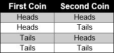
Using the results from the table, the following probabilities can be determined. The probability of tossing two heads is ¼. The probability of tossing 2 tails is ¼. The probability of tossing 1 head and 1 tail is ½. The game is unfair because the probability of each player winning is not equal.
Example #4: A teacher wants to choose 4 students from her class to participate on a special committee to plan the next dance. She lines them up alphabetically and has each student toss a coin. The first four students to toss a tail will be on the committee. Is this a fair way to select the committee?
Solution: This is not a fair way to select the committee because not all students have an equal chance of being chosen. Students at the back of the line may never get a chance to flip the coin.
Example #5: Heather and Sam play a game using a pair of dice. After they roll, they add the numbers together. If the sum is even, Heather wins. If the sum is odd, Sam wins. What is the probability of rolling an even sum? What is the probability of rolling an odd sum? Determine whether the game is fair. Explain why or why not.
Solution:
List all the possible outcomes. (First dice + Second dice)
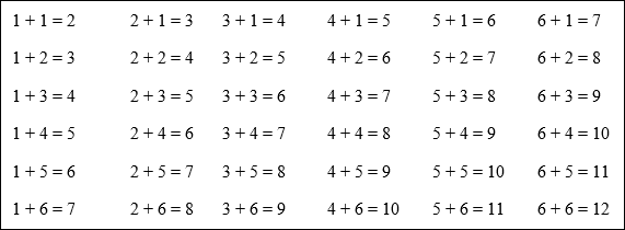 |
The first number listed represents the number on the first die and the second number represents the number on the second die. For example, 3 + 4 = 7, means a 3 was rolled on the first die and a 4 was rolled on the second die.
There are 36 possible outcomes.
Count the number of times an odd sum occurs.
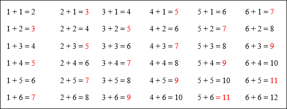 |
There are 18 combinations that result in an odd sum. The probability of rolling a pair of dice whose sum is odd is
Likewise, the probability of rolling a pair of dice show sum is even is
The game is fair because the probability of each player winning is equal.
A random number is a set of digits from 0 to 9 arranged in random order. A random number table is a listing of random numbers. Usually the random numbers are grouped in fives to make the table more readable. Random numbers can be used to help make fair decisions.
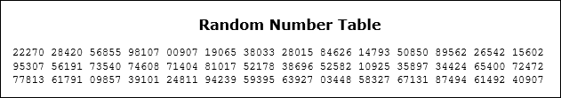 |
Example #6: A teacher wants to choose 5 students from her class to participate on a special committee to plan the next dance. She assigns each student in the class a two digit number from 01 to 25. How can the teacher use the random number table to choose the 4 students to be on the committee?
Solution: Pick a line from the random number table. We will use the first line. Read the digits from the table in consecutive pairs until you get the numbers for four of the students. Skip numbers like 27 and 84 since the do not represent any of the students.
 |
The first student chosen is student number 22. The next pair of number is 27, this number is skipped since no student has that number. The next student chosen is student 2 represented by 02. The next pair of numbers is 84, this number is also skipped since no student has that number. Continuing in this manner, the other students selected are 07 and 03. This method is fair because the numbers are generated randomly.
There are many random number generators available on the internet. Each time a fair decision has to be made a different random number table can be generated.
Stop! Go to Questions #1-6 about this section, then return to continue on to the next section.
Using Probability to Analyze Decisions
A table can be used to determine probabilities and the probabilities can then be used to evaluate decisions.
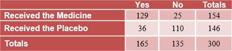
Example #1: A company is testing the effectiveness of a new cold medicine. Out of the 300 volunteers who had a cold, 154 were given the new cold medicine and 146 were given a placebo. A placebo is substance that has no active ingredients. It is used as a control in an experiment to determine the effectiveness of a medicinal drug. After 3 days, the volunteers were asked if there cold symptoms were gone. The results of the survey are shown in the table below.
 |
a) What is the probability that a volunteer reported their cold symptoms were gone given that he received the new cold medicine?
The first row of the table shows the number of volunteers who received the cold medicine. Out of the 154 who received the medicine, 129 reported that their cold symptoms were gone.
 |
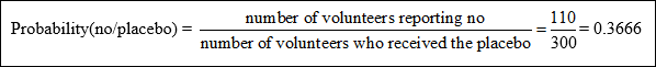
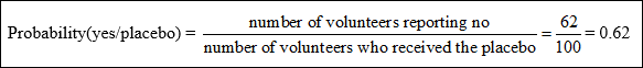
b) What is the probability that a volunteer received the placebo given reported his cold symptoms were not gone?
The second column of the table shows the number of volunteers who reported their cold symptoms were not gone. The second row represents the number of volunteers who received the placebo.
 |
c) The company decides to put the cold medicine on the market. Based on the results of the survey, did the company make a good decision?
Yes, the company made a good decision. The results of the survey show that about 84% of the people who were given the cold medicine no longer had any cold symptoms after 3 days. Also, about 75% of the volunteers who received the placebo did not experience relief from their cold symptoms.
Example #2: The results of another test are shown in the table below. Volunteers were asked to report whether their cold symptoms had disappeared after 4 days.
 |
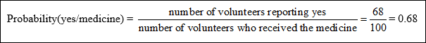
a) What is the probability that the cold symptoms disappeared in a volunteer who was given the medicine?
 |
b) What is the probability that a volunteer received the placebo and reported his cold symptoms were gone?
The second column of the table shows the number of volunteers who reported their cold symptoms were not gone. The second row represents the number of volunteers who received the placebo.
 |
c) Should the company market the new cold medicine? Explain
The cold medicine was only slightly more effective than the placebo. So, no the company should not market the cold medicine.
Stop! Go to Questions #7-12 about this section, then return to continue on to the next section.
STATISTICS |
Statistics is the collection, study, analysis, and interpretation of data. When data is collected and summarized, we can look for trends and try to make predictions based on these facts.
Surveys, Experiments and Observational Studies
Statistics involves the collection and analysis of data. In a statistical study, data is collected and used to make inferences, or general conclusions about a population characteristic or parameter. A population is all the members of a set. It is often impractical or impossible to collect data from every member of a population. You can often get good statistical information about a population by studying a sample of the population. A sample is a part of the population. If the sample is chosen carefully, the statistics for the sample can be used to make inferences about the larger population.
Suppose you want to know what percent of all the voters in your school district are in favor of a tax increase to build a new high school football stadium. It is almost impossible to ask the opinion of every single voter. So instead you will ask a sample of the voters in the school district. When choosing a sample, it is important to select an unbiased sample. A bias is an error that results when a part of the population is overrepresented or underrepresented. A sample is biased if its design favors certain outcomes. For example, going to a high school football game and asking 100 random fans whether they favored the building of a new stadium would be a biased survey. The fact that they are attending a football game would indicate their interest in the high school football program. An example of an unbiased survey would be conducting a telephone poll of 100 random voters in the school district asking if they were in favor of a tax increase to build a new football stadium. A random sample, in which members of the population are selected entirely by chance, reduces the possibility of selecting a biased sample.
There are several different types of statistical studies that can be used to collect data. We will look at surveys, observational studies and experiments.
In a survey, data is collected by asking members of the sample a set of questions. Surveys may involve being interviewed or answering a questionnaire. An example of a survey, is taking a poll to learn who people will vote for in an upcoming election.
In an experiment, the sample is divided into two groups. The experimental group undergoes a change, but the control group does not undergo a change. Comparisons are then made between the two groups. In an experiment, something is intentionally done to people, animals or objects and then the response is observed. An example of an experiment is selecting 100 people to test a new pain reliever. Fifty of the people are given the pain reliever and the other fifty people are given a placebo (a fake treatment). Data is then collected and analyzed to determine the effectiveness of the new pain reliever.
In an observational study, members of a sample are observed in such a way that they are not affected by the study. An example of an observational study would be to find 100 college students half of whom took a calculus class in high school and compare their grades in a college calculus class. The sample population being studied is measured as it is. No attempt is made to influence the results. Data is merely collected, analyzed and interpreted.
Stop! Go to Questions #13-19 about this section, then return to continue on to the next section.
Margin of Error
When conducting a survey, it is often impossible to survey everyone in the population. A margin of error applies when a population in not completely sampled. Thus, when you report the results of a statistical survey, you need to include the margin of error. The margin of error is a statistic expressing the amount of random sampling error in a survey’s results. For example, suppose you survey a group of high school students in which 55% of those surveyed said they participated in a sport. If given the margin of error is 4%, the likely interval that contains the percentage of high school students who participate in a sport is 51% to 59%. The lower number in the range is obtained by taking the percentage from the survey and subtracting the margin of error, (p – ME) 55% - 4% is 51%. Whereas the upper number in the range is obtained by taking the percentage and adding the margin of error (p – ME), 55% + 4% = 59%. The margin of error tells you the accuracy of the results of the survey. The greater the margin of error, the less accurate the survey.
Example #1: A recent survey reports that 43% of the voters favor candidate A with a margin of error of 3%. Find the likely interval that contains the percentage of voters who favor candidate A.
Take the percentage from the survey and subtract the margin of error, p – ME, 43% - 3% = 40%
Take the percentage from the survey and add the margin of error, p + ME, 43% + 3% = 46%
Thus, the likely interval that contains the percentage of the population who favor candidate A is 40% to 46%.
The margin of error is based on the size of the sample and the confidence level desired. A common confidence level is 95%. A confidence level of 95% means that 95% of the time, the percent of the population responding in the same way will be within the range of p – ME and p + ME. The formula to calculate the margin of error with a 95% confidence error is as follows:
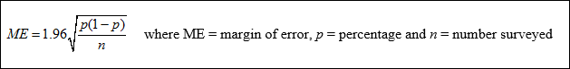 |
The coefficient 1.96 varies depending upon the desired confidence level. All of the examples in this unit will use a 95% confidence level.
Example #2: A recent survey of 1000 randomly selected adults from the United State showed that 54% of the people surveyed think the president is doing a good job. Find the margin of error rounded to the nearest whole percent. Then find an interval that is likely to contain the true population proportion.
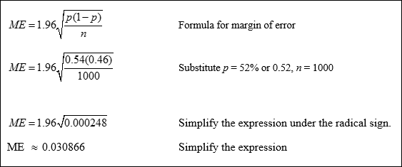 |
The margin of error is about 3%. Change to a percent by moving the decimal point two places to the left.
Find the interval that is likely to contain the true population proportion.
p – ME = 54% - 3% = 51%
p + ME = 54% + 3% = 57%
There is a 95% chance that the percent of people in the whole population that think the president is doing a good job is between 51% and 57%.
Example #3: In a recent survey of 450 high school students, 333 said that pizza was their favorite food served in the school cafeteria. Find the margin of error rounded to the nearest percent. Then find the interval that is likely to contain the true population proportion.
First calculate the percentage whose favorite food was pizza.
Find the margin of error.
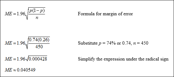 |
The margin of error is about 4%. Change to a percent by moving the decimal point two places to the left.
Find the interval that is likely to contain the true population proportion.
p – ME = 74% - 4% = 70%
p + ME = 74% + 4% = 78%
There is a 95% chance that the percent of students in the whole population whose favorite cafeteria food is pizza between 70% and 78%.
Example #4: In a recent survey, 68% of high school students said they preferred watching football to watching basketball. The margin of error was 4%. How many people were surveyed?
 |
About 523 students were surveyed.
Stop! Go to Questions #20-22 about this section, then return to continue on to the next section.
Measures of Central Tendency
Measures of central tendency are useful tools for representing statistical data. The most common measures of central tendency are mean, median and mode.
Mean: the average of a set of data (found by adding all the data together and dividing by the total number of elements).
Median: the middle number in the set when the elements are placed in order from least to greatest or greatest to least (if two numbers appear in the middle, those two numbers are added together and averaged).
Mode: the number that appears most often (there may be no mode, one mode, or more
than one mode).
Example #1: The scores on a recent test for an Algebra II class were 87, 74, 85, 87, 97, 74, 35, 86, 87 and 94. Find the mean, median and mode.
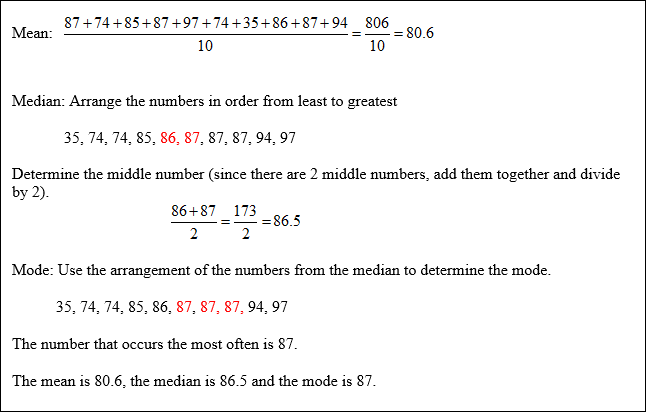 |
An outlier is a value that is extremely different from the rest of the data in the set. They can be misleading because they can affect measures of central tendency. In the example above the outlier is 35.
Example #2: Find the mean, median and mode from Example #1 when the outlier is not included. Describe the effect on each measure.
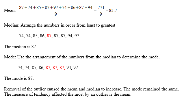 |
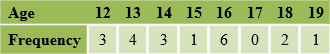
Example #3: Find the mean, median, and mode from a frequency table.
The following table represents the ages of club members attending a recent 4-H meeting. Find the mean, median and mode of the ages of the club members.
 |
Solution:
To calculate the ages of the members , notice there are 3 members whose age is 12, 4 members whose age is 13, 3 members whose age is 14 etc. ones, 10 twos, 5 threes, 3 fours and 1 six. The total ages of the members can be found as follows:
3(12) + 4(13) + 3(14) + 1(15) + 6(16) + 0(17) + 2(8) + 1(19)= 296
Find the total number of members: 3 + 4 + 3 + 1 + 6 + 0 + 2 + 1 = 20
Calculate the mean by dividing the total of the ages by the number of club members.
Mean =
Calculate the median by listing each age the number of time it occurs and find the middle number.
12, 12, 12, 13, 13, 13, 13, 14, 14, 14, 15, 16, 16, 16, 16, 16, 16, 18, 18, 19
Since there are 2 middle numbers, add them together and divide by 2.
Mode: Look at the frequency table to determine the mode. There are 6 club members whose age is 16. The mode is 16.
Stop! Go to Questions #23-31 about this section, then return to continue on to the next section.
Measures of Variation
A measure of variation is a measure that describes how spread out or scattered a set of data. It is also known as a measure of dispersion or a measure of spread. The three most common measures of variation are range, variance and standard deviation. Variance and standard deviation are measures of variation that indicate how much the data values deviate or differ from the mean.
Range: The difference between the greatest and least values in a set of data.
Example #1: The heights in inches of ten students are: 62, 60, 65, 59, 63, 61, 61, 64, 62, 64. Find the range of the data.
The maximum height is 65. The minimum height is 59.
Range: 65 – 59 = 6 ( Range = maximum height – minimum height)
Variance: The average of the squared differences from the mean of a set of data. Variance tells us how measured data vary from the average value of the set of data.
Standard deviation: A measure of how closely all of the data in a set of data surrounds the mean. Its symbol is σ (the Greek letter sigma). The symbol for the variance is σ2.
Steps to Finding Variance and Standard Deviation.
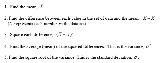 |
A low standard deviation indicates that the data points tend to be very close to the mean. A high standard deviation indicates that the data points are spread over a large range of values.
Example #2: Find the mean, variance and standard deviation for the following data set.
60, 40, 35, 45, 39
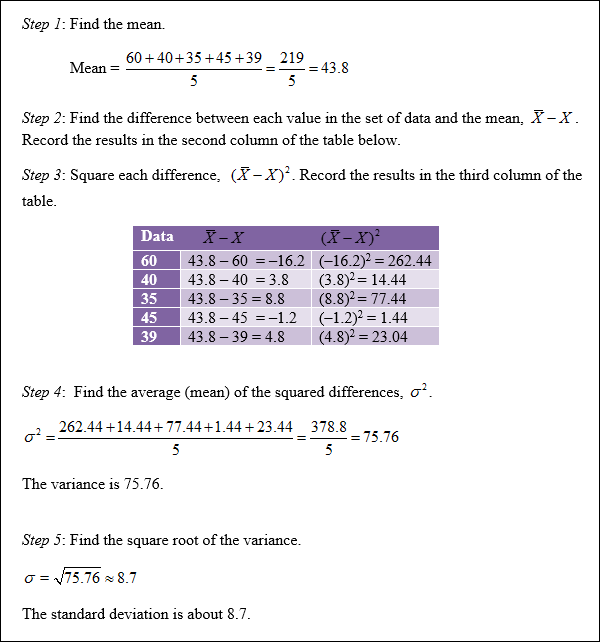 |
Example #3: Using a Frequency Table to Calculate the Mean and Standard Deviation of a Set of Data
When the amount of data is large, calculating the standard deviation can be time consuming. Using a frequency table will save some of the work.
Mrs. Hopper surveyed the 25 students in her Algebra II class to find the number of children in each of their families. The results are shown in the table below. (7 families had 1 child, 10 families had 2 children, etc.) Find the mean and the standard deviation of the number of children in the families.
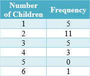 |
To calculate the number of children, notice there are 6 ones, 10 twos, 5 threes, 3 fours and 1 six.
The total count of the children is 1(5) + 2(11) + 3(5) + 4(3) + 6(1) = 60.
Calculate the mean by dividing the number 60 by the number of respondents,
Mean =
Find the difference between each value in the set of data and the mean, ![]() . Record the results in the second column of the table below.
. Record the results in the second column of the table below.
Square each difference, ![]() . Record the results in the third column of the table.
. Record the results in the third column of the table.
Add a 5th column to the table. Multiply the number is column 4 by their frequencies.
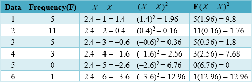 |
Find the average (mean) of the squared differences, σ2.
The variance is 1.36
The standard deviation, σ, is the square root of the variance.
The standard deviation is about 1.2 children.
Stop! Go to Questions #32-38 about this section, then return to continue on to the next section.
Normal Distributions
Many common statistics tend to have a normal distribution about the mean. Standardized test scores, heights of people, blood pressures and levels of production can all be represented by a normal distribution.
Normal distributions have these properties.
- The mean, median and mode are all equal.
- The graph of the curve is bell shaped.
- The maximum point on the curve is the mean.
- 50% of the values are less than the mean and 50% of the values are greater than the mean.
- About 68 % of the values are within 1 standard deviation of the mean.
- About 95% of the values are within 2 standard deviations of the mean.
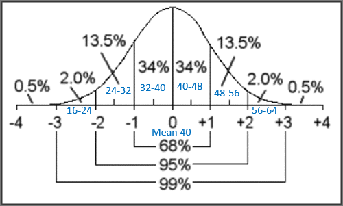
- About 99% of the values are within 3 standard deviations of the mean.
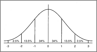
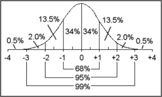 |
The numbers on the horizontal axis represent the number of deviations away from the mean. Thus, zero represents the mean of the data. + 1 represents one standard deviation above the mean, + 2 represents two deviations above the mean, etc. Likewise, -1 represents one standard deviation below the mean, -2 represents two deviations below the mean etc.
In a normal distribution, 34% of the data will be 1 deviation above the mean and 34% of the data will be 1 deviation below the mean. So a total of 68% of the data will be within 1 standard deviation of the mean. To find the range of values that lie within one standard deviation of the mean, take the value of the standard deviation and then find the mean plus the standard deviation, and the mean minus the standard deviation. A total of 95% of the data will be within 2 standard deviations of the mean. To find the range of values that lie with two standard deviations of the mean, you must multiply 2 times the standard deviation and then add and subtract that number from the mean. The same procedure is followed for finding the values that lie within three standard deviations or 99% of the values. The standard deviation would then be multiplied by 3.
Example #1: A normal distribution has a mean of 76 and a standard deviation of 6.
| a) Find the range of values that represent the middle 68% of the distribution. b) Find the range of values that represent the middle 95% of the data. c) Find the range of values that represent the middle 99% of the data. |
| a) Find the lower limit of the range by subtracting the standard deviation from the mean: 76 – 6 = 70 Find the upper limit of the range by adding the standard deviation to the mean: 76 + 6 = 82. Therefore, the range of the values that represents the middle 68% of the data are between 70 and 82, inclusive. b) To find the range of values that represent the middle 95% of the data you must be within two standard deviations of the mean. Multiply the standard deviation by 2: 2 × 6 = 12 Find the lower limit of the range by subtracting this value from the mean: 76 – 12 = 64 Find the upper limit of the range by adding this value to the mean: 76 + 12 = 88 Therefore, the range of the values that represents the middle 95% of the data are between 64 and 88, inclusive. c) To find the range values that represent the middle 99% of the data you must be within three standard deviations of the mean. Multiply the standard deviation be 3: 3 × 6 = 18 Find the lower limit of the range by subtracting this value from the mean: 76 – 18 = 58 Find the upper limit of the range by adding this value to the mean: 76 + 18 = 94 Therefore, the range of the values that represents the middle 99% of the data are between 58 and 94, inclusive. |
Example #2: A normal distribution has a mean of 40 and a standard deviation of 8. Find the probability that a value selected at random is in each of the given intervals.
| a) from 40 to 48 b) from 24 to 40 c) from 32 to 56 d) at most 48 |
Determine the values for three standard deviations above and below the mean.
| Mean: 40 One standard deviation above the mean: 40 + 8 = 48 Two standard deviations above the mean: 40 + 2(8) = 56 Three standard deviations above the mean: 40 + 3(8) = 64 One standard deviation below the mean: 40 – 8 = 32 Two standard deviations below the mean 40 – 2(8) = 24 Three standard deviations below the mean: 40 – 3(8) = 16 |
Place the numbers in order from smallest to largest and label with the appropriate standard deviation (SD)
 |
| a) From 40 to 48 represents the range from the mean to one standard deviation above the mean. Refer to the normal distribution graph to see that this represents 34% of the data. Therefore, the probability that a value selected at random is in the range 40 to 48 is 34% b) From 24 to 40 represents the range from 2 standard deviations below the mean to the mean. Refer to the normal distribution graph and add the corresponding percentages: 13.5% + 34% = 47.5%. Therefore, the probability that a value selected at random is in the range 24 to 40 is 47.5%. c) From 32 to 56 represents the range from 1 standard deviation below the mean to 2 standard deviations above the mean Refer to the normal distribution graph and add the corresponding percentages: 34% + 34% + 13.5% = 81.5% Therefore, the probability that a value selected at random is in the range 32 to 56 is 81.5%. d) At most 48, represents all percentages that are less than 1 standard deviation above the mean. Refer to the normal distribution graph and add the corresponding percentages: 0.5% + 2% + 13.5% + 34% + 34% = 84% Therefore, the probability that a value selected at random is at most 48 is 84%. |
Example #3: The scores on an Algebra II exam are normally distributed with a mean of 120 and a standard deviation of 15.
| a) What percentage of the students scored above 135 points? b) Out of 200 tests, how many students scored above 105 points? |
| Calculate the score for 1 standard deviation above the mean. The mean + the standard deviation is 120 + 15 = 135. Calculate the score for 1 standard deviations below the mean. The mean – 1 standard deviations is 120 – 15 = 105. |
It may be necessary to calculate 2 and 3 standard deviations above and below the mean depending upon the numbers given in the problem. But since 1 standard deviation above and below represented the numbers given in the problem, no additional calculations are needed.
| a) 135 represents one standard deviation above the mean. Refer to the normal distribution graph and add the percentages that are above one standard deviation. 13.5% + 2% + 0.5% = 16% Therefore 16% of the students scored above 135 points. b) 105 represents one standard deviation below the mean. Refer to the normal distribution graph and add the percentages that are to the right of one standard deviation below the mean: 34% + 34% + 13.5% + 2% + 0.5% = 84%. Therefore 84% of the students taken the test scored above 105 points. To calculate the number of student who scored above 105 points, multiply 200 students × 84%. 200 × 0.84 = 168 Therefore, 168 students scored above 105 points on the final exam. |
Stop! Go to Questions #39-42 to complete this unit.