RATIONAL EXPRESSIONS AND GRAPHS
 |
Unit Overview
In this unit you will work with rational expressions. You will begin by looking at rational functions in the context of joint, inverse, and combined variation. You will then take a functional approach to rational equations and explore the graph of such functions.
Inverse, Joint, and Combined Variation
In unit 2, you studied direct variation. In this unit, you will review direct variation and study other types of variations.
| Direct variation: two variables, x and y, have a direct variation relationship if there is a nonzero number k such that y = kx or k = y/x, k is the constant of variation. In a direct variation, as one quantity increases, the other quantity increases or as one quantity decreases the other quantity decreases. For example, an employee’s wages vary directly as the number of hours worked. The more hours that the employee works the more money he makes. |
Example #1: The variable y varies directly as x, and y = 12 when x = 3. Find x when y = 20.
|
Example #2: The length L that a spring will stretch varies directly with the weight W that is attached to the spring. If a spring stretches 12 inches with 15 pounds attached, how far will it stretch with 20 pounds attached?
The spring stretches 16 inches when 20 pounds are attached. |
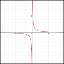
| Inverse variation: two variables, x and y, have inverse variation relationship if there is a nonzero number k, such that xy = k or y = |
Example #3: The variable y varies inversely as x, and y = 22.5 when x is 6.2.
|
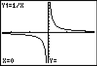
Look at the graphs below to see the location of each point on the graph of y = 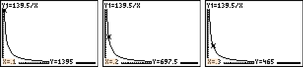 |
| Example #4: Twelve workers can complete a construction job in 8 days. How many workers are needed to complete the same job in 6 days. This is an inverse variation, as the number of workers increases the number of days required decreases.
|
Joint variation: (one quantity varies directly as two or more quantities) If y = kxz, then y varies jointly as x and z, and the constant of variation is k. |
| Example #5: When y varies jointly as x and z, write the appropriate joint-variation equation, and find y for the given value of x and z. y = –108 when x = –4 and z = 3, find y when x = 6 and z = –2
|
| Example #6: When y varies jointly as x and z, write the appropriate joint-variation equation, and find y for the given value of x and z. y = 15 when x = 9 and z = 1.5; find y when x = 18 and z = 3
|
| Example #7: The area (A) of a triangle varies jointly as the lengths of its base (b) and height (h). If A = 133 when b = 19 and h = 14, find A when b = 11.5 and h = 7. If A = 133 when b = 19 and h = 14, find A when b = 11.5 and h = 7.
|
| Combined variation: when more than one type of variation occurs in the same equation, z = |
| Example #8: z varies jointly as x and y and inversely as w. If z = 3 when x = 3, y = –2 and w = –4, find z when x = 6, y = 7, and w = –4.
|
For each of the following, state whether each equation represents a direct, joint, inverse or combined variation. Then name the constant of variation.
![]() Name the type of variation. Name the constant of variation. u = 8wz
Name the type of variation. Name the constant of variation. u = 8wz
The type of variation is "joint variation".
The constant of variation is 8.
"Click here" to check the answer.
![]() Name the type of variation. Name the constant of variation. xy = 6.5
Name the type of variation. Name the constant of variation. xy = 6.5
The type of variation is "inverse variation".
The constant of variation is 6.5.
"Click here" to check the answer.
![]() Name the type of variation. Name the constant of variation. y = 10x
Name the type of variation. Name the constant of variation. y = 10x
The type of variation is "direct variation".
The constant of variation is 10.
"Click here" to check the answer.
![]() Name the type of variation. Name the constant of variation. y =
Name the type of variation. Name the constant of variation. y = ![]()
The type of variation is "inverse variation".
The constant of variation is 5/8.
"Click here" to check the answer.
![]() Name the type of variation. Name the constant of variation. y =
Name the type of variation. Name the constant of variation. y = ![]()
The type of variation is "combined variation".
The constant of variation is 2/3.
"Click here" to check the answer.
![]() Name the type of variation. Name the constant of variation.
Name the type of variation. Name the constant of variation. ![]()
The type of variation is "direct variation".
The constant of variation is 3/4.
"Click here" to check the answer.
Stop! Go to Questions #1-13 about this section, then return to continue on to the next section.
Rational Functions and Their Graphs
Rational expression: a rational expression is the quotient of two polynomials. |
|
|
 |
|
To find the domain:
|
|
Example #1: Find the domain of
|
*Rational functions have asymptotes (a line that a curve approaches, but does not reach as its x or y values become very large or very small). They may also have holes in the graph (places where the function is undefined at specific x-values.)
To find all vertical and horizontal asymptotes use the following rules:
Vertical asymptotes: if x – a is a factor of the denominator but not a factor of the numerator, then x = a is the equation of the vertical asymptote of the graph. |
|
Horizontal asymptotes: let R(x) =
|
|
| Hole in the graph: if x – b is a factor of the numerator and the denominator, then there is a hole in the graph of the function at x = b. | |
| Let’s look at the graph of the rational function given in Example #1, and then test our rules. |
|||||
 |
|||||
|
|||||
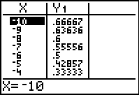
*Note: Visually, holes do not show up very well on a graphing calculator. |
|||||
|
|||||
| Thus, for the rational function, |
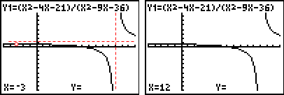
Example #2: Identify all asymptotes and holes in the graph of the following.
|
Example #3: Identify the domain restrictions and all asymptotes and holes in the graph of the following.
|
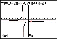
Let’s try one more.
Example #4: Identify the domain restrictions and all asymptotes and holes in the graph of the following.
|
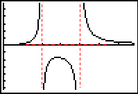
The following is the graph of a rational function with the asymptotes denoted by dashed lines.
y = |
vertical asymptote x = 2 |
horizontal asymptote y = 1 |
 |
To graph this function by hand on paper, you can use your calculator as an aid.
| a.) Enter the function into your calculator under Y=. | ||
b.) To find values to graph, you could use the TABLE feature,
|
Stop! Go to Questions #14-30 to complete this unit.