SOLVING POLYNOMIAL EQUATIONS
 |
Unit Overview
This unit is about solving polynomial equations by using variable substitution and by using the rational root theorem. The unit concludes with verifying and proving polynomial identities.
Solving Polynomial Equations by Using Variable Substitution and Factoring
One of the most important theorems in mathematics is the Fundamental Theorem of Algebra.
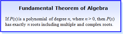 |
The polynomial, x4– 9x2 + 14 = 0, is a polynomial of degree 4 so it should have 4 roots. The roots may be real numbers, complex numbers, and/or the same number. These roots will be found in the following example.
If a polynomial has a degree of more than 2, variable substitution can be used find the roots.
Example #1: Solve for x: x4– 9x2 + 14 = 0
|
Example #2: Solve for z: z5 – 28z3 + 27z = 0
Therefore, the roots of the polynomial z5 – 28z3 + 27z = 0 are 0, 1, –1, |
Stop! Go to Questions #1-5 about this section, then return to continue on to the next section.
Rational Root Theorem
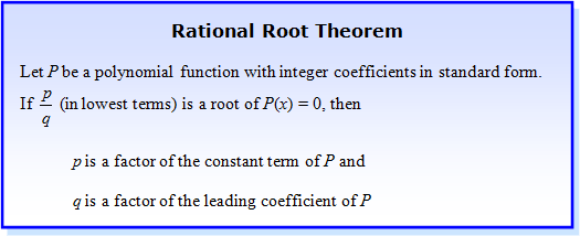 |
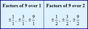
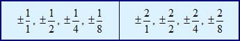
| Example #1: List all the possible rational roots of the function P(x) = 2x3– 11x2 + 12x + 9. According to the Rational Root Theorem, If p is a factor of the constant term, 9, and q is a factor of the leading coefficient, 2.
|
Let's practice determining the possible rational zeros of the polynomial, P(x) = 2x3– x2 + 2x + 5.
![]() Name the constant term. P(x) = 2x3– x2 + 2x + 5
Name the constant term. P(x) = 2x3– x2 + 2x + 5
5
"Click here" to check the answer.
![]() List the factors of the constant term. P(x) = 2x3– x2 + 2x + 5
List the factors of the constant term. P(x) = 2x3– x2 + 2x + 5
±1, ±5
"Click here" to check the answer.
![]() Name the leading coefficient. P(x) = 2x3– x2 + 2x + 5
Name the leading coefficient. P(x) = 2x3– x2 + 2x + 5
2
"Click here" to check the answer.
![]() List the factors of the leading coefficient. P(x) = 2x3– x2 + 2x + 5
List the factors of the leading coefficient. P(x) = 2x3– x2 + 2x + 5
±1, ±2
"Click here" to check the answer.
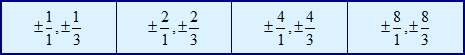
![]() List the possible rational roots. P(x) = 2x3– x2 + 2x + 5
List the possible rational roots. P(x) = 2x3– x2 + 2x + 5
"Click here" to check the answer.
Stop! Go to Questions #6-7 about this section, then return to continue on to the next section.
Solving Polynomial Equations Using the Rational Root Theorem
Note: The following examples are shown using a graphing calculator. The activities can be also be done using an online graphing program. Click here to navigate to the online grapher.
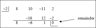
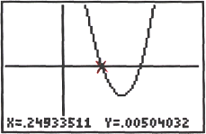
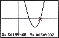
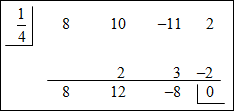
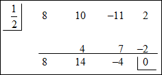
| Example #1: Find all of the rational roots of 8x3 + 10x2 – 11x + 2 = 0. According to the Rational Root Theorem,
|
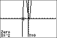
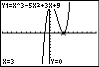
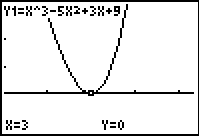
*When a polynomial function P(x) touches but does not cross the x-axis at (r, 0), then P(x) = 0 has a double root.
| For example: P(x) = (x – 3)(x – 3)(x+1) or P(x) = x3– 5x2 + 3x + 9 touches the x‑axis at (3, 0) but does not cross the x-axis there, as shown in the graphs below.
Therefore, 3 is a double root of P(x) = 0. |

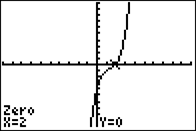
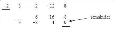
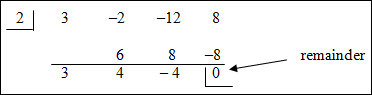
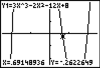
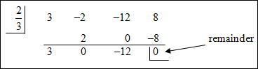
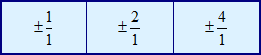
| Example #2: Find all of the rational roots of 3x3 – 2x2 – 12x + 8 = 0 According to the Rational Root Theorem,
|
Some polynomials do not have all rational roots. We can still find all the zeros of a function using some of the strategies already learned.
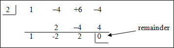
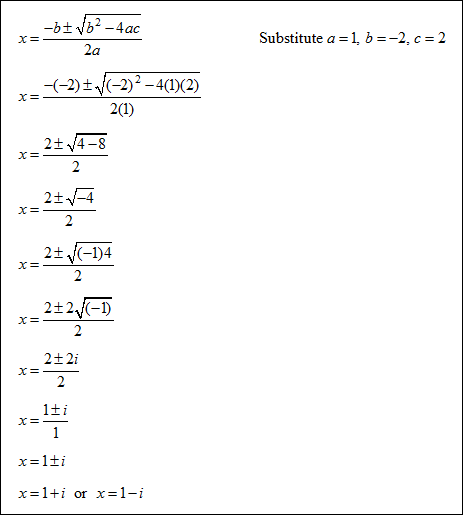
| Example #3: Find all of the roots of x3 – 4x2 + 6x – 4 = 0. According to the Rational Root Theorem,
|
Stop! Go to Questions #8-12 about this section, then return to continue on to the next section.
Proving Polynomial Identities
A polynomial identity is a statement of equality between two polynomials that is true for all values of the variable(s) for which the expression is defined.
Example #1: Check the polynomial identity (a + b)2 = a2 + 2ab + b2 by substituting a = 4 and b = 2.
|
Example #2: Prove the polynomial identity (a + b)2 = a2 + 2ab + b2 using algebraic operations.
|
Example #3: Check the polynomial identity a3 – b3 = (a – b)( a2 + ab + b2) by substituting a = 4 and b = 2.
|
Example #4: Prove the polynomial identity a3 – b3 = (a – b)( a2 + ab + b2) using algebraic expressions.
|
Stop! Go to Questions #13-33 to complete this unit.