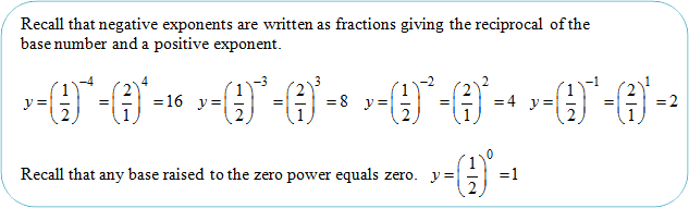
Exponential Growth and Decay

EXPONENTIAL GROWTH AND DECAY

Unit Overview
In this unit, we will look at a variety of applications that are modeled by exponential functions. Exponential functions model many scientific phenomena. Some applications of exponential functions include population growth, compound interest, and radioactive decay. Radioactive decay is used to date ancient objects found at archeological sites.

Exponential Functions

Consider each of the following functions.

y = x²		y = 2^x
This is a quadratic function because the base is a variable and the exponent is fixed.		This is an exponential function because the base is fixed and the exponent is a variable.

An exponential function is a function with the general form y = ab^x, a ≠ 0, b is a positive real number and b ≠ 1. In an exponential function, the base b is a constant. The exponent x is the independent variable where the domain is the set of real numbers.

There are two types of exponential functions: exponential growth and exponential decay.

In the function f (x) = b^xwhen b > 1, the function represents exponential growth.

In the function f (x) = b^x when 0 < b < 1, the function represents exponential decay.

For example:

a.) f (x) = 5^xwould represent exponential growth because b > 1. (b = 5)

b.) f (x) = 0.83^x would represent exponential decay because 0 < b < 1. (b = 0.83)

c.) f (x) = 0.5(3)^x would represent exponential growth because b > 1. (b = 3)

Example #1: Using a calculator and the exponential key (^), evaluate 4^x for x = 0.5.

Substitute the given value for x and evaluate.

4^x = 4^0.5 = 2

Example #2: Evaluate 5^x for x = 4.

Substitute the given value for x and evaluate.

5^x = 5⁴= 625

The expression 100 ⋅ 2ⁿ is called an exponential expression because the exponent n is a variable, and the base 2 is a fixed number. The base of an exponential expression is commonly referred to as the multiplier.

Example #3: Evaluate 10(2)^x for x = 3.

Substitute the given value for x and evaluate.

10(2)^x = 10(2)³= 10(8) = 80

*Recall that exponents take priority over multiplication.

Example #4: Evaluate 8(3)^x^{− 1} for x = 5.

Substitute the given value for x and evaluate.

8(3)^x^{− 1} = 8(3)^{5 − 1} = 8(3)⁴ = 8(81) = 648

Exponential Functions (03:50)

Stop! Go to Questions #1-5 about this section, then return to continue on to the next section.

Graphing Exponential Functions

As with other functions, ordered pairs can be used to graph an exponential function. In this section we'll examine graphs that show exponential growth and exponential decay.

Graphing an Exponential Function with b > 1

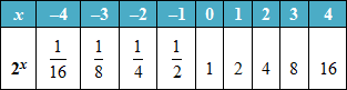
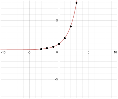
The first example will show the graph of exponential growth because the base is greater than 1. (b = 2)

Example #1: Graph y = 2^x.

Step 1: Make a table of values. Choose x-values and substitute the values in the function and calculate y.

Step 2: Graph the ordered pairs and connect the points with a smooth curve.

*Notice that the graph grows slowly at first, but then grows exponentially as the x‑values increase.

The graphs of exponential functions showing growth have the following characteristics:

The graphs of functions of the form y = b^x, where b > 1 all have the same shape as the graph shown above.
This graph is always increasing. The graph rises faster and faster as x gets larger. Notice that the value of the function is always positive throughout its domain. Therefore, the range is all positive numbers.
When y-values gets closer and closer to the x-axis as x equals smaller negative numbers, the graph will not intersect the x-axis. Therefore, the x-intercept does not exist.
The y-intercept is 1. (Remember the y-intercept is the y-value when x = 0.)

Exponential Growth -- Cell Divisions (02:33)

Graphing an Exponential Function with b < 1

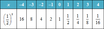
The next example will show the graph of exponential decay because the base is a number between 0 and 1. (b = 1/2)

Example #2: Graph .

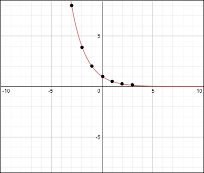
Step 1: Make a table of values. Choose x-values and substitute the values in the function and calculate y.

Step 2: Graph the ordered pairs and connect the points with a smooth curve.

The graphs of exponential functions showing decay have the following characteristics:

The graphs of functions of the form y = b^x, where 0 < b < 1 all have the same shape as the graph shown above.
This graph is always decreasing. The graph falls as x gets larger. Notice that the value of the function is always positive throughout its domain. Therefore, the range is all positive numbers.
When y-values gets closer and closer to the x-axis as x equals larger numbers, the graph will not intersect the x-axis. Therefore, the x-intercept does not exist.
The y-intercept is 1. (Remember the y-intercept is the y-value when x = 0.)

Graphing an Exponential Function with y = ab^x

The factor a in y = ab^x can stretch or compress the graph of the parent graph y = b^x. If a < 0, the graph will reflect across the x-axis.

The graphs of y = 2^x (in blue) and y = 3(2)^x (in red) are shown below. Each y-value of y = 3(2)^x is 3 times the corresponding y-value of the parent function y = 2^x.

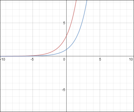The graph of the parent function y = 2^x is stretched by a factor of 3. Note the y-intercept of y = 3(2)^x is 3. The domain of the function is the real numbers and the range is all positive numbers.

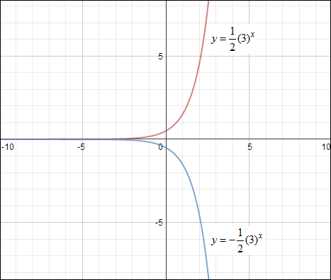
Example #3: Compare the characteristics of the graphs of the given functions.

The graphs of

(in red) and

(in blue) are shown below.

In the graph,

, the

compresses the graph of the parent graph

by a factor of

. The y-intercept is

. The range is all positive numbers, so y > 0.

In the graph of

, the

reflects the graph of the parent graph

across the x-axis and compresses it by a factor of

. The y-intercept is

. The range is all negative numbers, so y < 0.

Now, let's review the characteristics of exponential graphs.

What is the domain of y = 4^x ?

The real numbers.

"Click here" to check the answer.

*The domain of ALL exponent functions is the real numbers.

What is the range of y = 3^x?

The range is y > 0.

"Click here" to check the answer.

What is the y-intercept of y = 2^x ?

The y-intercept is 1.

"Click here" to check the answer.

What is the y-intercept of y = ?

The y-intercept is –1/3.

"Click here" to check the answer.

What is the range of y = ?

The range is y < 0.

"Click here" to check the answer.

*The range is all negative numbers because the negative sign caused the graph to reflect over the x-axis.

Stop! Go to Questions #6-13 about this section, then return to continue on to the next section.

Applications of Exponential Growth and Decay

To solve exponential growth and decay problems, apply the rules given in the table.

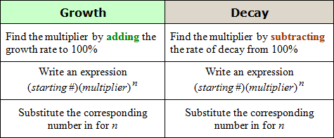Example #1: Find the multiplier for the rate of exponential growth, 4%.

                     Since this represents exponential growth, add 100% + 4% = 104%.

                     Express the percent as a decimal. 104% = 1.04

                     The multiplier is 1.04

Example #2: Find the multiplier for the rate of exponential decay, 9.3%.

                     Since this represents exponential decay, subtract 100% – 9.3% = 90.7%.

When a quantity grows by a fixed percent at regular intervals, the pattern can be represented by the following function.

Now, let's see how these rules apply to some common real-world applications of growth and decay.

Example #3: Suppose that you invested $1000 in a company’s stock at the end of the current year and that the value of the stock was predicted to increase at a rate of about 15% per year. Predict the value of the stock, to the nearest cent, at the end of the five years, and then ten years.

At the end of the 5th year:

Step #1: Calculate the multiplier.

100% + 15% = 115% or 1.15 is used for the multiplier.

Step #2: Use the given information and y = abⁿ to calculate the predicted value of the stock.

The starting number (a) is 1,000, the multiplier (b) is 1.15, and the time (n) is 5 years.

y = abⁿ

y = (1,000)(1.15)⁵ = $2,011.36

Therefore, the value of the stock is predicted to be $2011.36 in five years.

At the end of the 10th year:

The multiplier (1.15) was calculated in the previous problem.

The starting number is 1000, the multiplier is 1.15, and the time is 10 years.

y = abⁿ

y = (1,000)(1.15)¹⁰ = $4,045.56

Therefore, the value of the stock is predicted to be $4,045.56 in ten years.

Deriving the Equation for Annual Compound Interest (02:19)

Using a Graphing Calculator to Calculate Annual Compound Interest (02:38)

Example #4: Suppose that you buy a car for $15,000, and that its value decreases at a rate of about 8% per year. Predict the value of the car, to the nearest cent, after 4 years, and then after 7 years.

Value after 4 years:

Step #1: Calculate the multiplier.

100% – 8% = 92% or 0.92 is used for the multiplier.

Step #2: Use the given information and y = abⁿ to calculate the predicted value of the stock.

The starting number (a) is 15,000, the multiplier (b) is 0.92, and the time (n) is 4 years.

y = abⁿ

y = (15,000)(0.92)⁴ = $10,745.89

Therefore, the car will be worth $10,745.89 after 4 years.

Value after 7 years:

The multiplier (0.92) was calculated in the previous problem.

The starting number is 15,000, the multiplier is 0.92, and the time is 7 years.

y = abⁿ

y = (15,000)(0.92)⁷ = $8,367.70

Therefore, the car will be worth $8,367.70 after 7 years.

Doubling and Tripling

The following example demonstrates exponential growth when the original amount is repeatedly multiplied by a positive number, called the growth factor.

The growth factor is determined by adding 100% and the rate of growth.

If an amount is doubled, this means that 100% is added to 100%, so the multiplier will become 200% or 2.

If an amount is tripled, then the multiplier will be 300% or 3.

Example #5: Thirty rabbits are introduced to a secluded area with no predators. Assume that the rabbit population doubles every six months. How many rabbits will be in the area after three (3) years?

a.) Since the population doubles twice a year, in 3 years it will have doubled 6 times. There are 6 time periods (3 years = 6 half years). (n = 6)

b.) There are 30 original rabbits. (a = 30)

c.) The rabbits are doubling every 6 months. The multiplier for doubling is 2. (b = 200% = 2)

y = abⁿ

y = 30 × 2⁶ = 1920

In 3 years, there will be 1920 rabbits.

If the rabbit population tripled every 6 months, how many would be in the area after three years?

21,870 [y = 30(3)⁶]

"Click here" to check the answer.

Compound Interest

Compound interest is modeled by an exponential function.

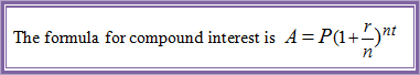A = the total amount of an investment

P = principle

r = annual interest rate

n = number of times the interest is compounded per year

t = time in years

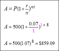
Example #6: Find the final amount of a $500 investment after 8 years at 7% interest compounded annually, quarterly, monthly and daily and compare the results.

Principal P = 500 Rate r = 7% = 0.07 Time t = 8

Compounded Annually (The amount is compounded once a year, n = 1).

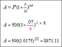
Compounded Quarterly (The amount is compounded every 3 months in a year; that is, 4 times a year; thus, n = 4).

Compounded Monthly (The amount is compounded every month in a year; that is, 12 times a year; thus, n = 12).

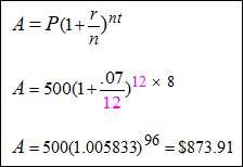Compounded Daily (The amount is compounded every day in a year; that is, 365 times a year; thus, n = 365).

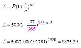Summarizing the results in a table, we can make a quick comparison of the amounts.

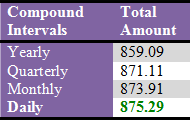Which type of compounding is most profitable?

Compounding Daily

"Click here" to check the answer.

Money in the Bank: Compound Interest (06:18)

Stop! Go to Questions #14-30 about this section, then return to continue on to the next section.

Below are additional educational resources and activities for this unit.

Click on the icon to find and practice topics for this unit.

Graphing Exponential Functions Worksheet 1

Graphing Exponential Functions Worksheet 2