CURVE FITTING AND QUADRATIC INEQUALITIES
In this unit you will find a quadratic function that exactly fits three data points. You will also investigate how quadratic regression can be used to process real-world data, and then used to make predictions. You will also write, solve and graph a quadratic inequality in one and two variables.
Curve Fitting
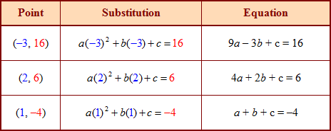
It is possible to find a quadratic function that fits a set of data points. To find a, b, and c in the function f (x) = ax2 + bx + c:
| 1.) write a system of three linear equations using the given points 2.) set up a matrix equation and solve
|
 into matrix A.
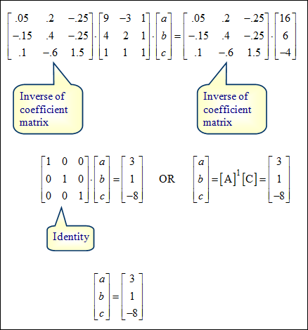
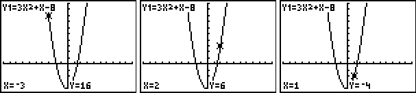
See the three graphing calculator windows below to verify.
 |
Stop! Go to Questions #1-3 about this section, then return to continue on to the next section.
Quadratic Regression
Quadratic regression is a process by which the equation of a parabola is found that “best fits” real-world data. A graphing calculator can be used to perform a quadratic regression and make predictions. The following examples illustrates the technique for a TI‑83, a TI83Plus, or a TI84 Plus.
If a graphing calculator is not available, click here for a link to a Quadratic Regression Applet.
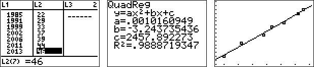
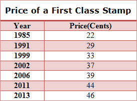
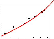
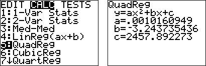
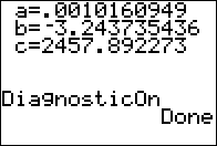
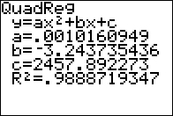
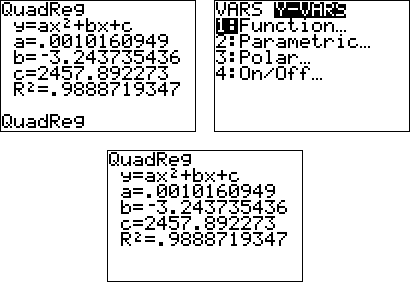
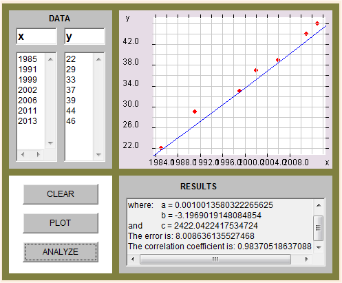
Example #1: The table below shows the price of a first class stamp over the years. Use a graphing calculator to find the quadratic regression equation for this data.
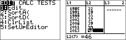
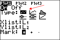
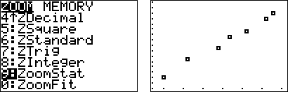
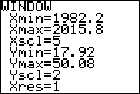
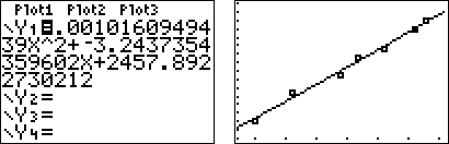
Enter the data for two lists, L1 representing the year and L2 representing the price. (L1, L2) Then examine the data points to see what kind of graph the data is suggesting.
|

Predicting Future Prices |
Now that the regression equation is determined, it can be used to predict the price of first class postage in other years.
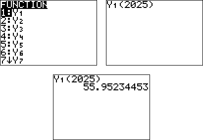
| Example #2: Predict the cost of a first class postage stamp in the year 2025 using the data stored in the graphing calculator. From the home screen, press
|
The same method can be used to see how the outcomes match the already known cost of stamps.
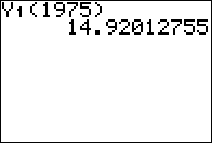
| Example #3: Calculate the cost of a first class postage stamp in the year 1975 using the data stored in the graphing calculator and compare that value to the actual cost of the stamp. From the home screen, press
The regression equation gives a price of 15 cents. The actual price of a first class postage stamp in 1975 was 13 cents ... pretty close! |
This method can also be used to find the best fit for linear, exponential and polynomial functions. By comparing the correlation coefficients it can be determined what type of function best fits the data.
To prepare the calculator for future use, clear all lists.
Stop! Go to Questions #4-7 about this section, then return to continue on to the next section.
Quadratic Inequalities
To solve a quadratic inequality:
| 1.) factor the quadratic 2.) the solutions represent the critical points on the x-axis and divide the axis into sections that must be tested. 3.) test each section to determine what area to shade. |
If the inequality is < or ≤, then the solution will be connected with the word “and”.
Example #1:
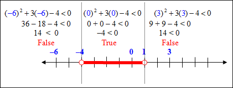
x2 + 3x − 4 < 0
Choose test points from each section of the graph to determine which area needs to be shaded. We will test –6, 0, and 3.
Based on the results of the testing, the solution to this quadratic will be greater than –4 AND less than 1. This can be written as (–4 < x < 1). |
||||||||||
If the inequality is > or ≥, then the solution will be connected with the word “or”.
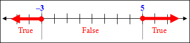
Example #2: x2 − 2x − 15 ≥ 0
Choose points from each section to test for validity.
The testing shows true statements for x-values less than –3 or x-values greater than 5. Therefore the solution to this quadratic inequality is x ≤ –3 or x ≥ 5. |
|||||||||||||||||||
Stop! Go to Questions #8-11 about this section, then return to continue on to the next section.
Graphing Quadratic Inequalities
| 1.) the quadratic must be in the form of y = a(x − h)2 + k where the vertex is located at (h, k) 2.) graph the vertex and set up a table to find other points on the curve, choose two x‑values greater and two x-values less than the x-value of the vertex 3.) replace the chosen points into the inequality to find y-values 4.) graph each point and connect them 5.) shade the appropriate region |
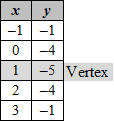
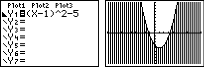
Example #1: y ≤ (x − 1)2 − 5
|
||||||
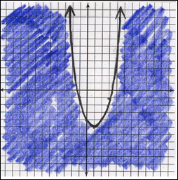
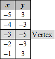
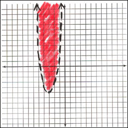
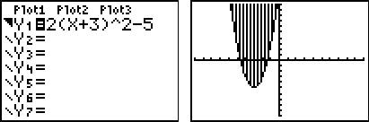
Example #2: y > 2(x + 3)2 − 5
|
||||||
Let’s take a look at the graphs above using the graphing calculator.
To graph y ≤ (x − 1)2 − 5, enter
To graph y > 2(x + 3)2 − 5, enter
*You will still need to determine if the line is solid or dotted by your knowledge of inequalities. |
If the quadratic function is not in vertex form, there are two methods that can be used to find the vertex.
| 1.) Complete the square to put the equation in vertex form or 2.) Use the equation |
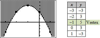
| Example #3: Graph y ≥ −2x2 − 4x + 3 Method 1 Using Vertex form
Method 2: Find the x-coordinate of the vertex first, then substitute to find the y‑coordinate.
The vertex is (–1, 5). To graph the quadratic inequality, choose x-coordinates near the x-coordinate of the vertex, and substitute them into the quadratic equation to find the corresponding y‑coordinates.
The graph is a solid line because the inequality symbol is greater than or equal (≥). The graph is shaded above the curve because a greater than sign is in the inequality symbol (≥) and the quadratic equation is in standard form. |
Now let's practice graphing inequalities. Click here to view the activity.
Stop! Go to Questions #12-25 to complete this unit.