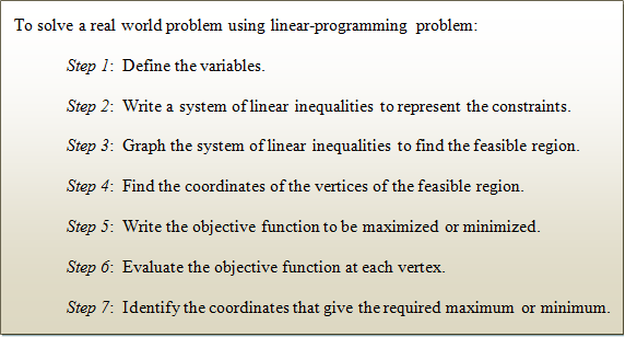
SOLVING SYSTEMS OF LINEAR INEQUALITIES
Unit Overview
Linear inequalities can be used to model real-world problems. For example, a linear inequality can be used to model the distance that a car with given fuel-economy ratio can be driven using no more than twenty-two gallons of gasoline. In this unit you will solve and graph linear inequalities in two variables, and then write and graph a set of constraints for a linear-programming problem.
System of Linear Inequalities
A system of linear inequalities is a collection of linear inequalities in the same variables. The solution is any ordered pair that satisfies each of the inequalities.
To graph a system of linear inequalities
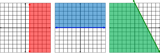
1.) graph each inequality individually, decide which half-plane to shade
2.) after all inequalities are graphed, the solution is the intersection of all the individual solutions.
Example #1: y ≥ –x – 1 The intersection of both graphs occurs in the darkened area because of the shading. |
 |
|
|
 |
![]() The Intersection (03:58)
The Intersection (03:58)
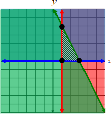
Now let’s add a third line, x < 1, to the system of inequalities and examine the intersection of all three lines.
Example #2: y ≥ –x – 1 Shading occurs above the red line, to the right and below of the blue line and to the left of the green line. |
 |
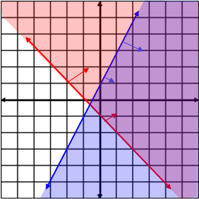
To determine a system of inequalities from a graph:
1.)
find the equations for the boundary lines: ≤, ≥ will be a solid line |
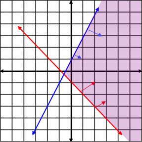
Example #3: The blue line represents x ≥ 0 and the red line represents
|
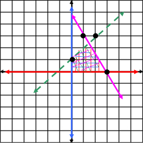 |
Choose one of the given points, (2, 3), to find the equation. y – 3 = 1(x – 2) The pink line contains the points (3, 0) and (1, 3) so the slope is |
Stop! Go to Questions #1-4 about this section, then return to continue on to the next section.
Linear Programming
Linear programming is a method used to find a minimum or maximum value of some quantity. Often this quantity is cost or profit and used in business applications. Constraints are the inequalities used in linear programming. Feasible region is the solution set. Objective function is the function to be maximized or minimized. |
If there is a maximum and minimum value of the objective function, it always occurs at one of the vertices of the feasible region.
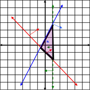
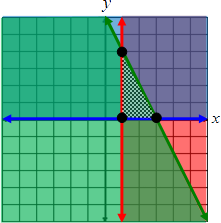
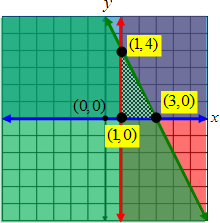
Example #1: Graph the following constraints. Name the coordinates of the vertices of the feasible region. Find the maximum and minimum values for the objective function P = 3x + y. The intersection of the boundaries are the vertices of the feasible region.
Step 2: Find the coordinates of the vertices of the feasible region.
The intersection of the boundaries are the vertices of the feasible region. The polygon formed is a triangle with vertices at (1, 4), (3, 0) and (1 ,0). P = 3x + y At (1, 4): P = 3(1) + 4 = 7 At (3, 0): P = 3(3) + 4 = 9 (Maximum) At (1, 0): P = 3(1) + 4 = 3 (Minimum) P has a maximum value of 9 at (3, 0) and a minimum value of 3 at (1, 0). |
Let's review what we've learned thus far about linear programming. In the next few questions and/or statements, read through and fill in the blanks about linear programming. Use terms from the given word bank. After deciding which terms fit best, click to reveal the answers.
 |
![]() To find the feasible region for a linear programming problem,
To find the feasible region for a linear programming problem,
solve the system of linear _________ called ____________.
inequalities, constraints
"Click here" to check the answer.
![]() The points within the feasible region are the __________ of the system.
The points within the feasible region are the __________ of the system.
solution set
"Click here" to check the answer.
![]() The corner points of the polygon formed are the _________ of the feasible region.
The corner points of the polygon formed are the _________ of the feasible region.
vertices
"Click here" to check the answer.
![]() The function to be maximized or minimized is called the __________.
The function to be maximized or minimized is called the __________.
objective function
"Click here" to check the answer.
![]() What significant values always occur at the vertices of the feasible region?
What significant values always occur at the vertices of the feasible region?
maximum and minimum values
"Click here" to check the answer.
 |
y ≥ 10 - She wants to make at least ( ≥ ) 10 large arrangements. x + y ≤ 50 - She wants to make at total of no more than ( ≤ ) 50 large arrangements.
The objective function that will represent the maximum profit is:
Since the maximum value is 910, the crafter should make 15 small wreaths and 35 large wreaths to gain maximum revenue. |
 Example #2: A crafter is making two sizes of wreath arrangements. The crafter charges $14 for the small arrangement and $20 for the large. She wants to make at least 15 small and 10 large arrangements with a total of no more than 50 arrangements. Let x represent the number of small arrangements, and let y represent the number of large arrangements. How many of each should she make to maximize her revenue?
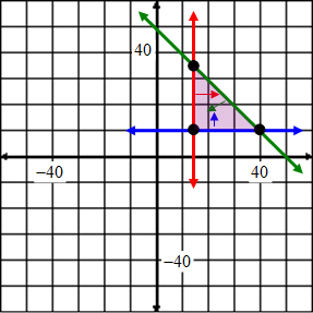
Stop! Go to Questions #5-23 to complete this unit.