Course Overview
In this course students will begin by reviewing basic algebra and geometry topics. They demonstrate fluency in operations with real numbers, vectors and matrices; represent and compute with complex numbers; use fractional and negative exponents to find solutions for problem situations; describe and compare the characteristics of the families of quadratics with complex roots, polynomials of any degree, logarithms, and rational functions. Students investigate rates of change, intercepts, zeros and asymptotes of polynomial, rational, and trigonometric functions graphically and with technology; identify families of functions with graphs that have rotation symmetry or reflection symmetry about the y-axis, x-axis, or y = x. They solve problems with matrices and vectors, solve equations involving radical expressions and complex roots, solve 3 by 3 systems of linear equations, and solve systems of linear inequalities; solve quadratic expressions, investigate curve fitting, and determine solutions for quadratic inequalities. They investigate exponential growth and decay and use recursive functions to model and solve problems; compute with polynomials and solve polynomial equations using a variety of methods including synthetic division and the rational root theorem; solve inverse, joint, and combined variation problems; solve rational and radical equations and inequalities; and describe the characteristics of the graphs of conic sections. They analyze the behavior of arithmetic and geometric sequences and series. Students use permutations and combinations to calculate the number of possible outcomes recognizing repetition and order; compute the probability of compound events, independent events, and dependent events. They use descriptive statistics to analyze and interpret data, including measures of central tendency and variation.
In some of the units, a graphing calculator will be useful. It is recommended that the graphing calculator be at least a TI-83 model.
LINEAR EQUATIONS
Unit Overview
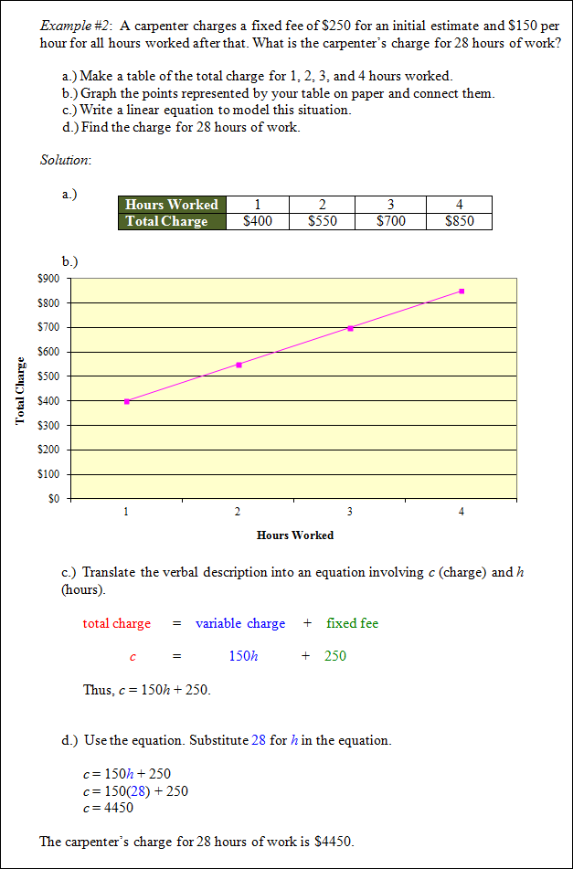
An equation that has a graph that is a line is called a linear equation. In this unit you will analyze linear equations in two variables using tables and graphs. By working with rate of change you will understand how the slope of a line can be interpreted in real world situations. Linear equations will be graphed using the slope and y-intercept. You will write a linear equation in two variables given sufficient information. Finally you will write an equation for a line that is parallel or perpendicular to a given line.
Tables and Graphs of Linear Equations
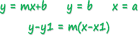
y = mx + b is called a linear equation and the graph is a straight line.
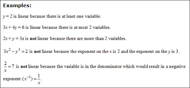
For an equation to be linear, the following must apply:
-There must be at least one variable, and at most 2 variables.
-The exponent on any of the variables must be equal to 1 (no more, no less).
When variables represented in a table of values are linearly related and there is a constant difference in the x-values, there is also a constant difference in the y-values.
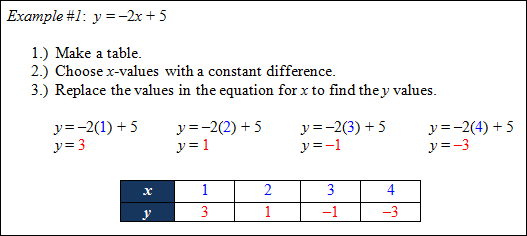
In a linear relationship, a constant difference in consecutive x-values results in a constant difference in consecutive y‑values.
![]() Linear Equations and Slope (15:01)
Linear Equations and Slope (15:01)
Application (Income)
Stop! Go to Questions #1-14 about this section, then return to continue on to the next section.
Rates of Change
A rate of change is a rate that describes how one quantity changes in relationship to another quantity.
Let's see how this works.
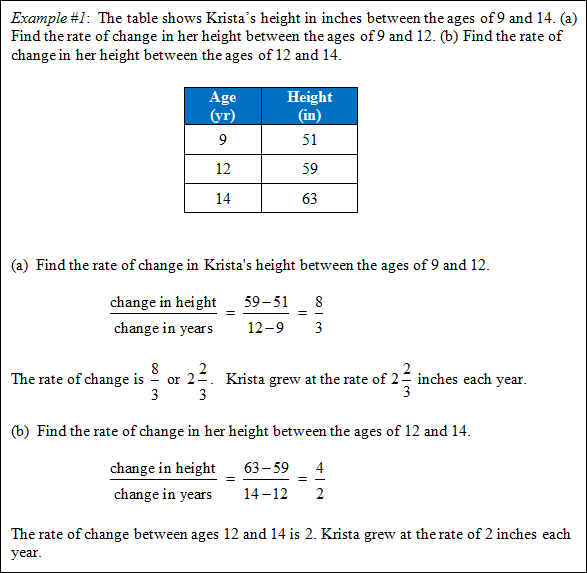
Find the Rate of Change Using a Table
In the first example, the rate of change in Krista's height is examined.
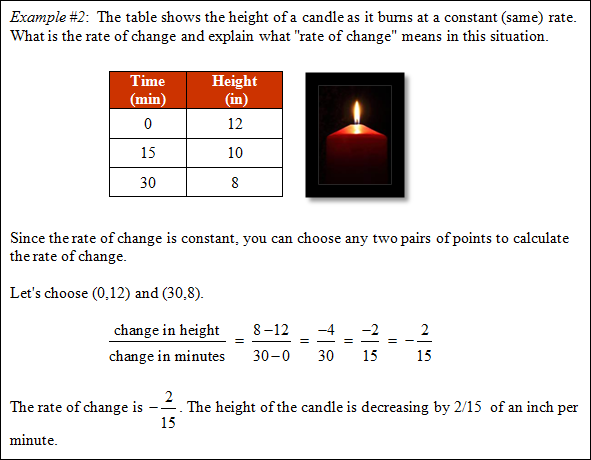
In this example the rate of change of a burning candle is examined.
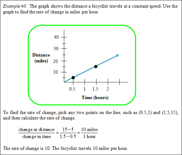
Find the Rate of Change Using a Graph
In this example the bicyclist's constant speed is examined as a rate of change.
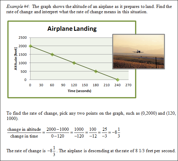
In this example rate of change in an airplane's height from the ground is examined as it descends to land.
![]() Slope-Intercept Form: An Introduction (04:47)
Slope-Intercept Form: An Introduction (04:47)
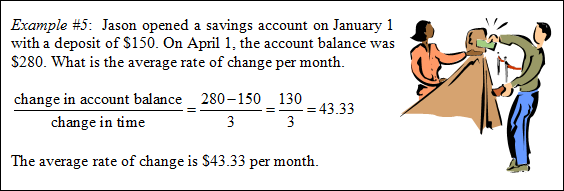
Average Rate of Change
Stop! Go to Questions #15-17 about this section, then return to continue on to the next section.
Slopes and Intercepts
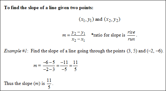
The slope of a line refers to the steepness and direction of the line and is found by finding the change in vertical units (y) divided by the corresponding change in horizontal units (x).
The slope of a line is a rate of change. Slope = ![]()
There are four (4) types of slopes.
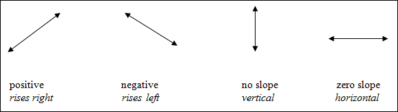
The slope of a line can be thought of as "RISE OVER RUN"; that is, "rise" parallel to the y-axis (change in y) over "run" parallel to the x-axis (change in x). Let's examine this further.
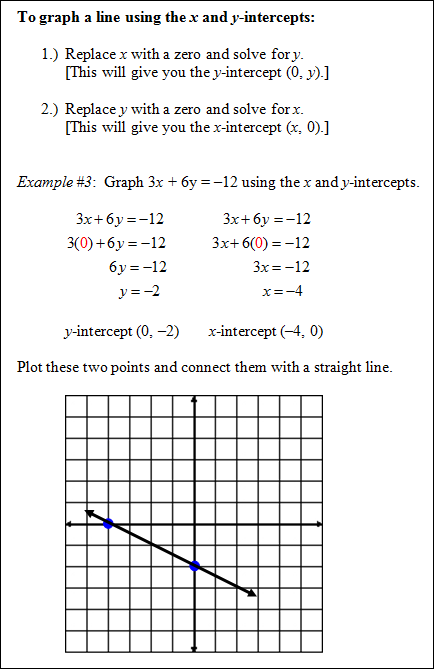
y-intercept: the point at which the line crosses the y-axis (0, y)
x-intercept: the point at which the line crosses the x-axis (x, 0)
slope-intercept form of a line: y = mx + b (m = slope, b = y-intercept)
standard form of a linear equation: Ax + By = C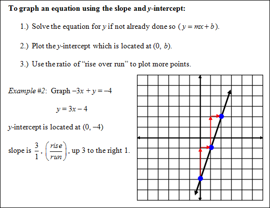 |
 |
Stop! Go to Questions #18-27 about this section, then return to continue on to the next section.
Linear Equations in Two Variables
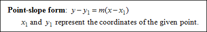
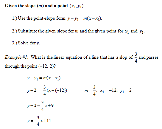
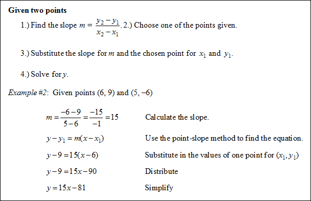
To find a linear equation using point-slope form:
![]() The Point-Slope Equation (01:16)
The Point-Slope Equation (01:16)
To find a linear equation using point-slope form:
Stop! Go to Questions #28-31 about this section, then return to continue on to the next section.
Equations of Horizontal and Vertical Lines
Recall that the slopes of horizontal and vertical lines are special cases.
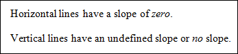
In this section we will discuss the equation of both of these lines and how to graph each.
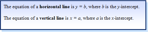
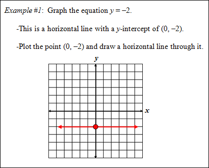
Equation of a Horizontal Line
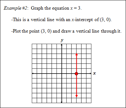
Equation of a Vertical Line
Stop! Go to Questions #32-33 about this section, then return to continue on to the next section.
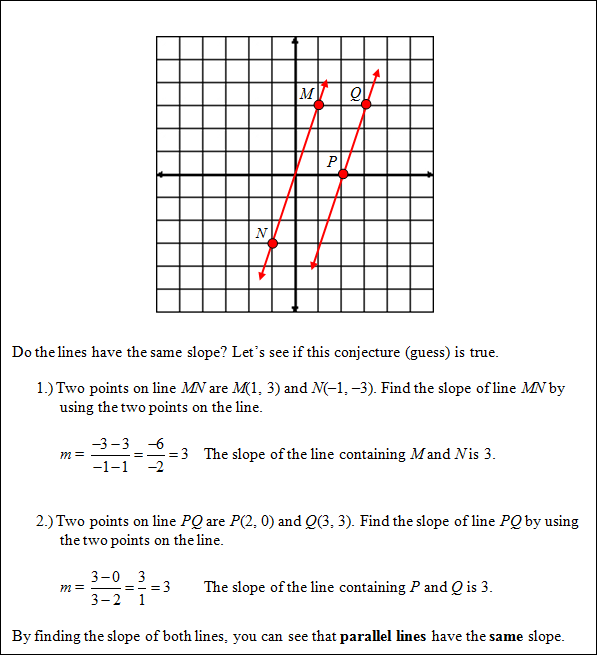
Parallel and Perpendicular Lines
Lines that never intersect are called parallel lines. There is a special relationship between parallel lines. Study the graph below and see if you can figure out what the special relationship is.
![]() Making Comparisons with Equations (02:56)
Making Comparisons with Equations (02:56)
Parallel lines have the same slope.
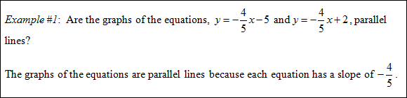
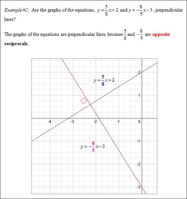
Perpendicular lines have opposite reciprocal slopes.
![]() What is the slope of a line that is parallel to y = –4x + 5?
What is the slope of a line that is parallel to y = –4x + 5?
The slope of the parallel line is ?4.
"Click here" to check the answer.
![]() What is the slope of a line that is perpendicular to y = (3/2)x – 7?
What is the slope of a line that is perpendicular to y = (3/2)x – 7?
The slope of the perpendicular line is the opposite reciprocal, ?2/3.
"Click here" to check the answer.
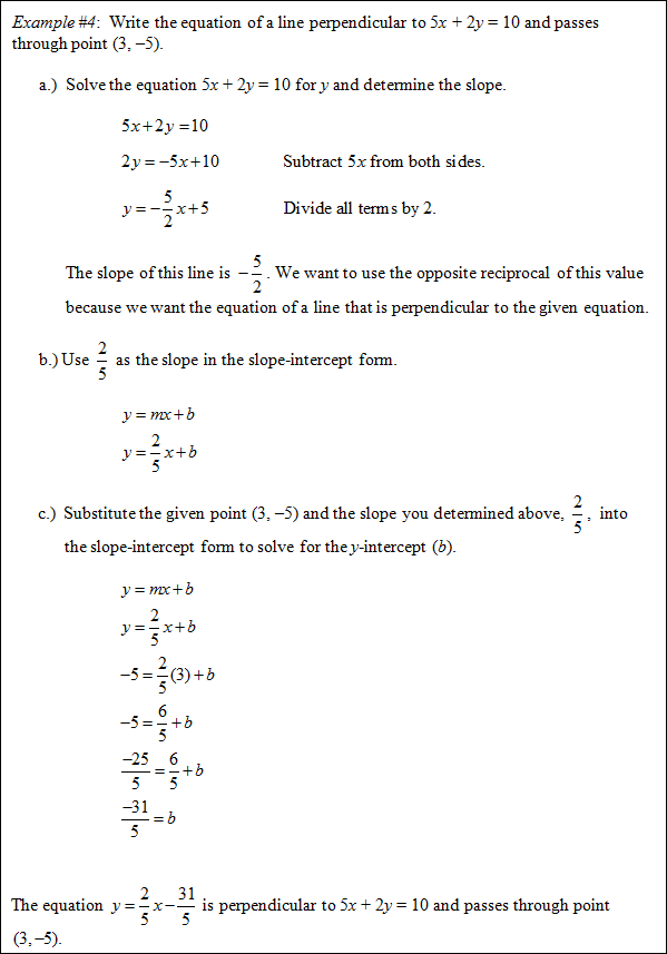
This knowledge provides us with the ability to write equations of lines that are parallel to or perpendicular to the lines of given equations and containing a certain point.

When working with linear equations, sometimes they are given in standard form and need to be expressed in slope-intercept form. In this case, solve the equation for y and proceed onward. This is shown in the next example.
![]() Converting Standard Form to Slope-Intercept Form (02:27)
Converting Standard Form to Slope-Intercept Form (02:27)
Let's finish with a quick quiz.
![]() What is the slope of a line that is parallel 2x – 4y = –3?
What is the slope of a line that is parallel 2x – 4y = –3?
The slope of the parallel line is 1/2.
"Click here" to check the answer.
![]() What is the slope of a line that is perpendicular to x – 3y = 5?
What is the slope of a line that is perpendicular to x – 3y = 5?
The slope of the perpendicular line is –3.
"Click here" to check the answer.
Stop! Go to questions #34-40 to complete this unit.