Graphing
Linear Functions
Unit Overview
In this unit, students will be able
to:
·
graph linear
functions in slope-intercept and standard form by finding solutions
·
identify
solutions for 2-variable functions
·
graph one
variable equations
Key Concepts
·
graphing solutions
for linear functions
Connection to
previous units
·
Unit 6: Functions → Linear Functions
·
Unit 7: Proportional Relationships → Linear Functions
Ohios Learning Standards
·
8.F.2 Compare properties of two functions each represented
in a different way (algebraically, graphically, numerically in tables, or by
verbal descriptions). For example, given a linear function represented by a
table of values and a linear function represented by an algebraic expression,
determine which function has the greater rate of change.
·
8.F.4 Construct a function to model a linear relationship
between two quantities. Determine the rate of change and initial value of the
function from a description of a relationship or from two (x, y) values, including
reading these from a table or from a graph. Interpret the rate of change and
initial value of a linear function in terms of the situation it models, and in
terms of its graph or a table of values
Calculators
·
Here is a link
to the Desmos scientific calculator that is provided for the Ohio State
Test for 8th Grade Mathematics in the spring.
·
You are
strongly encouraged to use the Texas Instruments TI-30XIIS handheld scientific
calculator. It is extremely user
friendly.
Linear Function
·
A linear function is a two-variable equation (usually x and y) that
forms a straight line when graphed
·
A linear function most commonly written in two forms:
o
Slope-intercept form (y =mx + b,
where m and b are numbers), where y is by itself on one side of the equation. Here are several examples
§ y = -5x
§ y = 2x + 3
§ ![]()
o
Standard form (Ax + By = C, where
A, B, and C are numbers), where x and y are on the same side of the equation. Here are several examples:
§ x + y = 6
§ 2x + 4y = 10
§ x 2y = 20
·
A solution
to a linear function is any ordered pair that makes the equation true.
·
A Linear function has an infinite number
of solutions.
·
The graphed line of a linear function is a visual representation of all of its solutions.
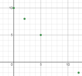
Example A: Lets look at an example:
o
x + y = 10
|
solutions |
Checking
the solutions for x + y
= 10 |
|
(5, 5) |
5 + 5
= 10 |
|
(2, 8) |
2 + 8
= 10 |
|
(0, 10) |
0 + 10
= 10 |
|
(12, -2) |
12 + (-2)
= 10 |
When graphing those solutions, notice that they
form a straight line:
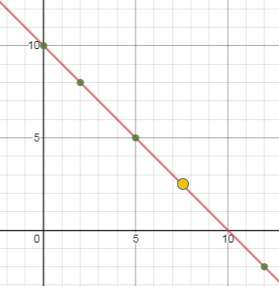
When graphing the entire equation, x + y = 10, a
line shows every ordered pair solution that makes the equation true. In this case, every ordered pair on the line
adds up to 10, including ordered pairs with decimals like (7.5, 2.5).
Example B: Lets look at another example, this time in
slope-intercept form:
o
y = 2x 1
|
solutions |
Checking
the solutions for y = 2x 1 |
|
(5, 9) |
9 = 25
1 |
|
(1, 1) |
1 = 21
1 |
|
(0, -1) |
-1 = 20
1 |
|
(3, 5) |
5 = 23
1 |
When graphing those
solutions, notice that they form a straight line.
When graphing the entire equation, y = 2x − 1, a
line shows every ordered pair solution that makes the equation true, including a ordered pairs with decimals like (2.5,
4).
HOW TO
GRAPH LINEAR EQUATIONS
·
The traditional algebraic process for graphing a linear function is:
o
1st: Find at
least two ordered pairs (points)
that are solutions for the function (using an x-y table).
o
2nd: Graph those
ordered pairs and draw a line
through them.
· Example C: Graph this slope-intercept form function: y = -4x + 6
1st: find two points that are solutions.
Since y is by itself, you
should pick
any number to put in for x, then solve for y. I suggest using 0 and 1 for x:
|
x |
y |
|
0 |
? |
|
1 |
? |
y = -40+6 à y = 6
y = -41+6 à y = 2
|
x |
y |
|
0 |
6 |
|
1 |
2 |
2nd: graph those two points, then draw
a line through them.
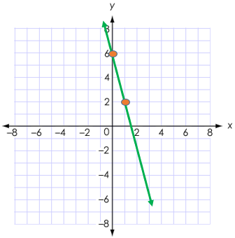
o
This line represents all solutions for y = -4x + 6
§ Solutions such as
(2, -2), (3, -6), (1.5, 0) and (-1, 10) all fall on this line.
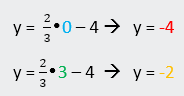
· Example D: Graph this slope-intercept form function:![]()
1st: find two points that are solutions.
Since y is by itself, you
should pick
any number to put in for x, then solve for y. Since you have a fraction, I suggest you use
0, as well as the denominator of the fraction (to avoid getting a fraction
answer to graph).
put in for x, then solve for y. I
suggest using 0 and 1 for x:
|
x |
y |
|
0 |
? |
|
3 |
? |
|
x |
y |
|
0 |
-4 |
|
3 |
-2 |
2nd: graph those two points, then draw
a line through them.
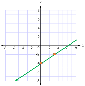
o
This line represents all solutions for ![]()
§ Solutions such as ![]() and (6,
0) all fall on this line.
and (6,
0) all fall on this line.
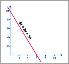
·
Example E: Lets
look at a function in standard form: 2x + 4y = 12
o
First, find two points. Since y
is not by itself, I suggest putting in 0 for x, then solving for y. Then
putting in 0 for y, then solve for x:
|
x |
y |
|
0 |
? |
|
? |
0 |
2x + 4y = 12
20 + 4y = 12
4y = 12
y = 3
2x + 4y = 12
2x + 40 = 12
2x = 12
x = 6
|
x |
y |
|
0 |
3 |
|
6 |
0 |
o
This line represents all solutions for 2x + 4y = 12
§ Solutions such as (1,
2.5), (2, 2), (3, 1.5) and (-2, 4) all fall on this line.
For a
further explanation of graphing linear equations:
Lets practice
graphing equations.
Checking Solutions
·
To check if an ordered pair is a solution to a function, you can
either:
o
Graph the function, and see if the point is on the line
o
Substitute the ordered pair into the function
and see if it makes the equation true.
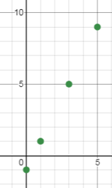
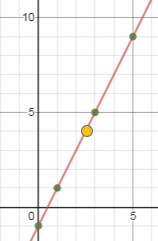
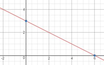
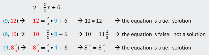
Example F: For the
function, ![]() which ordered
pairs are solutions?
which ordered
pairs are solutions?
A. (9,
12) B. (8, 10) ![]()
I first graphed the function, as well as the points.

You will notice
that (9, 12) and![]() are solutions
since they are both on the line. (8, 10)
is not a solution, since it is not located on the line.
are solutions
since they are both on the line. (8, 10)
is not a solution, since it is not located on the line.
We can also check
if those ordered pairs are solutions by substituting the x and y values into
the function:
For a
further explanation and practice on checking solutions for linear equations:
Lets practice checking
solutions for functions.
Graphing
One-Variable Equations: linear equations
sometimes use just one variable.
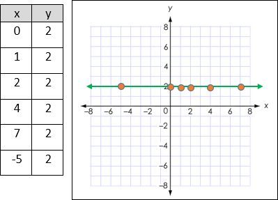
Example G: Graph y = 2
·
For this equation, there
are no requirements of the x-coordinate, but all of the solution points on the
line have 2 as a y-coordinate. Here are
a few:
·
A shortcut for graphing y = 2 is to go to 2 on the y-axis and draw
a horizontal line through it.
·
This equation is a function
o
each input (x) has just one
output (y).
o
No x-value has two different y-values.
o
It also passes the Vertical
Line Test.
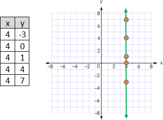
Example H: Graph the
equation, x = 4.
·
In this case, all the x-values must be 4.
·
The y-values can be anything.
·
A shortcut for graphing x = 4 is to go to 4 on the x-axis and draw
a vertical line through it.
·
This equation is NOT a function
o
one input (the x-value of 4)
has multiple different outputs
o
This line also does not pass
the vertical line test, since it is a vertical line.
For a
further explanation on one-variable linear equations:
Lets practice working with one-variable equations.